Predicting the Severity of Major Power Outages in the U.S.
Analysis by Pratham Aggarwal
Introduction
Power outages disrupt millions of lives, which raises pressing issues like public safety and emergency response to economic stability. A power outage may seem like a simple inconvenience like losing the chance to finish a show on Netflix, but its real impact goes far beyond that. In severe situations, a power outage can disable critical medical equipment, shut down heating or cooling during extreme weather, interrupt communication systems used by first responders, halt transportation services, and cause widespread economic losses for businesses and communities.
Some of the major columns for the data and their descriptions are shown below. For descriptions of all other columns, please visit here.
| Column | Description |
|---|---|
| dur_hours | Duration of the power outage in hours (calculated from outage start and restoration times). |
| customers.affected | Number of customers impacted by the outage event. |
| demand.loss.mw (megawatt) | Amount of electricity demand lost (in megawatts) during the outage. |
| population | Population of the state where the outage occurred. |
| poppct_urban (%) | Percent of the state population living in urban areas. |
| res.price (cents/kWh) | Residential electricity price in cents per kilowatt-hour. |
| pc.realgsp.state (usd) | Per-capita real gross state product (an economic indicator) in US dollars. |
Summary statistics of some variables that intuitively contribute most to the power outage are shown below.
Note: dur_hours is calculated by taking the difference between outage_restore and outage_start.
| dur_hours | customers.affected | demand.loss.mw (megawatt) | population | poppct_urban (%) | res.price (cents/kWh) | pc.realgsp.state (usd) | |
|---|---|---|---|---|---|---|---|
| count | 1476 | 1056 | 804 | 1476 | 1476 | 1464 | 1476 |
| mean | 43.7546 | 144117 | 543.399 | 1.31474e+07 | 80.9457 | 11.971 | 49387.5 |
| std | 99.0654 | 288110 | 2226.49 | 1.14772e+07 | 11.8922 | 3.09008 | 11828 |
| min | 0 | 0 | 0 | 559851 | 38.66 | 5.65 | 31111 |
| 25% | 1.70417 | 9700 | 4 | 5.3109e+06 | 74.57 | 9.5775 | 43056 |
| 50% | 11.6833 | 71661.5 | 175.5 | 8.82341e+06 | 84.05 | 11.5 | 48323 |
| 75% | 48 | 150000 | 400 | 1.94029e+07 | 89.81 | 13.85 | 53622 |
| max | 1811.88 | 3.24144e+06 | 41788 | 3.92965e+07 | 100 | 34.58 | 168377 |
To better understand these events, this project uses the Major Power Outage Events dataset, which records 1,535 power outages in the United States. Each outage has around 57 columns of information. This wide range of information motivates the central question of this project:
What factors influence how long a major power outage lasts, and can we predict outage duration using the available data?
Understanding and predicting outage duration can help policymakers and the general public prepare for emergency needs, allocate resources effectively, and plan according to outage severity.
Data Cleaning and Exploratory Data Analysis
To prepare the data for analysis several cleaning steps were taken to clean and standardize the data. First goal was to convert units properly, fix columns names, handel how date and time are stored and remove redundant information in the dataset. Since data was in .xlxs format it was converted to .csv using google sheets. Then we created a deep copy of the data to preserve the orginal raw information. First five rows were deleted because they contained some metadata, which was disrupting tabular data expectations for our analysis. Since units are crucial to this analysis, we drop the unit column and merge it with the header following the format: <col_name> (<unit>) (provided the units exist for the columns). Column names were converted into lowercase letters for convenience To keep our analysis handy we divided the variables into three major categories: categorical, numeric and datetime variables. All numeric variable were converted to float to avoid typecasting issues during model preperation. Moreover datetime variables like month, year, time were conveted to pandas datetime format using pd.to_datetime(). Therefore all datetime variables were merged into two unique columns called outage_start and outage_restore.Target variable (dur_hours) was prepared by taking the difference between outage_restore and outage_start further dividing by 3600 to convert into hours.
hurricane.names is not useful information for our analysis hence we drop that columns. Since other columns like cause.category and cause.category.detail tell us why outage happened, dropping hurricane.names won’t affect our model performance. obs was just an index columns hence we dropped it as well. variable (units) was dropped since we merged this information with columns headers. postal.codes was just US state names written in abbreviation, so we drop it.
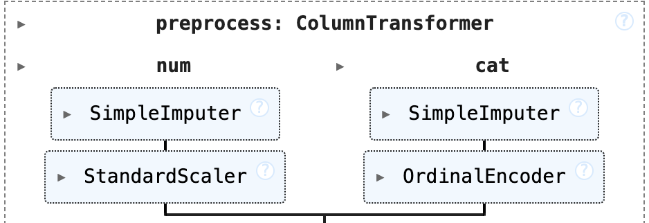
Missing values in the dataset were imputated using the preprocessing pipeline shown above. Numerical features like (anomaly.level (numeric),demand.loss.mw (megawatt),customers.affected) were passed through sklearn.SimpleImputer that replaced NaNs with median for each columns. We particularly replaced with median, because while doing Exploratory Data Analysis majority columns showed skewed towards right behavior, therefore median imputation became a better choice than mean imputation as median are less sensitive to outliers than mean.Later, the numerical varaibles are passed through StandardScalerdata into z-score. This is an important step as this will ensure that higher values of one feature would not dominate the ones with numerical lower value, ensuring a consistent analysis. Similarly categorical features were passed through sklearn.SimpleImputer that replaced NaNs with the most frequent category. Later OneHotEncoding was performed on categorical variables, essentially converting these categories into numbers. Note: Alternative imputation methods, including probabilistic and random sampling approaches, were explored. However, these techniques tended to inject noise and reduce predictive stability, so they were not used in the final preprocessing pipeline.
first five rows and columns of our cleaned dataset as follows:
| u.s._state | nerc.region | climate.region | anomaly.level (numeric) | climate.category | cause.category | |
|---|---|---|---|---|---|---|
| 0 | Minnesota | MRO | East North Central | -0.3 | normal | severe weather |
| 1 | Minnesota | MRO | East North Central | -0.1 | normal | intentional attack |
| 2 | Minnesota | MRO | East North Central | -1.5 | cold | severe weather |
| 3 | Minnesota | MRO | East North Central | -0.1 | normal | severe weather |
| 4 | Minnesota | MRO | East North Central | 1.2 | warm | severe weather |
Univariate Analysis
The below choropleth map shows the average duration of power outages in hours by U.S states. Darker regions indicate longer periods of power outage while lighter ones indicate on regions which recover power quicker than darker ones. The map shows diverse avergae otage durations across US states. The states in Northeast and Midwest tend to have higher and persistent power outages whereas Southern and Western states on average show shorter power outage durations. This observation is driven by various factors like climate exposure, infrastructure of the states, population density and other confounding variables not found in the dataset.
Bivariate Analysis
The boxplot below compares outage duration across different cause.categories, which explains us about how severity of power outage when depending on severity of the cause. Severe weather and fuel supply emergencies tend to produce longest an most variable outages, having many outliers. In contrast the intentional attacks and islanding generally shows lower outage duration. This analysis shows that cause of an outage plays an important role in determining how long the outage would last, hence making it an important feature to include.
Interesting Aggregates
| urban_bin | count | mean | median |
|---|---|---|---|
| Very Low | 296 | 41.36 | 9.43 |
| Low | 319 | 59.55 | 35.00 |
| Medium | 276 | 29.53 | 6.32 |
| High | 315 | 51.39 | 12.00 |
| Very High | 270 | 33.36 | 5.74 |
The aggregation tables paints a good picture of how outage severity varies across different levels of urbanizaton, which reveals some important patterns. States with lower urabanization experience longer periods of power outage. This supports our general understanding, since less urabanized places have inadequate infrastructure and limited urgency of restoration. On the contrary urabanized places, though have frequent outages, however they restore back quicker than lower urabanized places. This gives us a solid context on how urbanization influences power outage durations.
Assessment of Missingness
Based on the dataset the column which is most likely to be NMAR (Not Missing at Random) is
demand.loss (megawatt) During large severe outages, reporting systems are often deprioritized which increases the likelihood that the larger (unobserved) values of outages are missing. This further means that missing may be directly related to the variable itself (the definition of NMAR).
To frame it as MAR (Missing at Random) further information on why the values are missing would be needed. This additional information could be wind speed, precipitation, some disaster report or reporting system failure is needed. If these factors can convey some correlation with the missingness in demand.loss (megawatt) then MAR can be justified.
We test the following two hypothesis to for assessment of missingness in our data.
Missingness Hypothesis 1:
- H0: missingness in
anomaly.levelis independent of total water percentage (pct_water_tot (%)) - H1: missingness in
anomaly.levelis dependent on total water percentage (pct_water_tot (%)) - TS: Kolmogorov-Smirnov statistic, since KDE of both categroies is very similar mean/median would’nt suffice.
- Result: Failed to reject H0 (pval = 0.8247 , alpha = 0.05) Missingness appears to be random with respect to water percentage. Our general expectation says that it should be dependent on climate variable like anomally.level, but the analysis says the otherwise signaling a weaker effect of water percentage.
Missingness Hypothesis 2:
- H0: missingness in
anomaly.levelis independent of commercial electricity sales (com.sales (megawatt-hour)) - H1: missingness in
anomaly.levelis dependent on commercial electricity sales (com.sales (megawatt-hour)) - TS: Kolmogorov-Smirnov statistic, since KDE of both categroies is very similar mean/median would’nt suffice.
- Result: Reject H0 (pval = 0.0 , alpha = 0.05) Missingness appears to be random with respect to utility contribution, which is opposite to our general expectations, since commercial electricity sales would not influence climate anomally level. This appears to be more of a correlational result instead of causal outcome.
Hypothesis Testing
We will perform Permutation Testing to investigate the following:
- H0: outage duration is independent of climate category (using the encoding True if
climate.categoryis normal) - H1: outage duration is dependent on climate category.
- TS: Kolmogorov-Smirnov statistic, since KDE of both categroies is very similar mean/median would’nt suffice.
- Result: Failed to reject H0 (pval = 0.0557 , alpha = 0.05) Hence we have no statistical evidence that climate category influences outage duration (suprising result, but acceptable since power outages depend on weather more than climate). This result must not be taken very seriously, because it is very close to alpha, if we had more information (less nans) we may yeild opposite result.
Framing a Prediction Problem
The project will predict the duration (hours) of a major power outage, framing as a regression problem where target variable is dur_hours. Duration was chosen because outage duration is the most pressing factor when it comes to operationalizing the “severity” of a power outage as it has direct strong implications for emergency planning, resource allocation etc. To evaluate the model performance, we will be using the Mean Absolute Error as the primary metric. MAE is selected because it very easy to interpret and it is robust to outliers relative to metrics like Root Mean Squared Error (RMSE). By focussing on MAE, our model would be used as a better day to day tool to predict the severity of general outages.
Baseline Model
The baseline model we used is multiple linear regression to predict the severity of power outage, operationalized by duration of outage in hours. Linear Regression would be a simple starting point to understand regression limitations and need for feature engineering. It would be a great benchmark for later more complicated models. As a review we have: for baseline model we will include all the features to predict outage duration. Specifically, dataset contains 6 nominal features (state and region/category variables), 0 ordinal features, and 46 quantitative features (including anomaly.level, all numeric measures, percentages, economic indicators, population stats, densities, and duration).
As in data cleaning section we reiterate the following, Numerical features like (anomaly.level (numeric),demand.loss.mw (megawatt),customers.affected) were passed through sklearn.SimpleImputer that replaced NaNs with median for each columns and then it was passed through StandardScaler to convert them into z-scores. This is an important step as this will ensure that higher values of one feature would not dominate the ones with numerical lower value, ensuring a consistent analysis. Similarly categorical features were passed through sklearn.SimpleImputer that replaced NaNs with the most frequent category. Later OneHotEnoding was performed on categorical variables. Baseline’s objective would be understand the correlation between variables.
After running the preprocessing pipeline and training the model, we obtain an MAE of 37.50 on the training set and 46.04 on the test set. While these results are not ideal, the model still performs better than a naïve mean baseline, which produces MAE = 47.5 (train) and MAE = 53.85 (test). Although the model improves upon the baseline, its overall performance remains weaker than desired. This suggests that additional feature engineering, hyperparameter tuning, or exploring alternative model architectures may be needed to achieve stronger predictive accuracy.
Final Model
Feature Engineering
We applied log1p() to variables such as number of customers affected, demand loss, population and population densities. These variables are massivley large and very sparse, since outage duration typically grows in diminshing returns fashion with some feature, rather than linearly. Log tranform are expected to reduce the skewness of the data, in other words would decrease the variance. This would tune features to mimic how outages scale in real world.
The original columns were replaced with log tranformed ones.
Furthermore to bring meaning to the categorical variables for our model, we adopt a strategic middle ground technique between OrdinalEncoding and OneHotEncoding. cause_avg, state_avg, clim_avg were added, these were created by having group them and taking the median of dur_hours.
Furthermore, we added interaction features such as anomally_x_loss, urban_x_customers, cause_x_anomally to account for compouding effects. Outage duration is not solely dependent upon single, instead it is impacted due to various factors. For example accounting for high demeand loss during an unfortunate weather event or a large customer outage occuring in a highly urbanized ares. These interactions give model much better understanding of multiplicative nature of outage severity, seen in real life.
RandomForestRegressor
We chose RandomForestRegressor for this problems, intital experiments showed that model overfitted heavily, producing low train error however maintaing high test error. To reduce overfitting we simplify our model by dropping high correltion features. We plot the correlational matrix before and after removing features having absolute correlation greater than 0.9. doing this we get the following correltional maps before and after results.
Looking at the both the figures, we see that multicollinearity decreased after removal. Note: the dark digonal represents self-correlation (always 1) as expected.
The following features were removed due to excessive correlation or limited predictive value:
res.price (cents / kilowatt-hour)com.price (cents / kilowatt-hour)ind.price (cents / kilowatt-hour)res.sales (megawatt-hour)com.sales (megawatt-hour)ind.sales (megawatt-hour)total.sales (megawatt-hour)res.customerscom.customersind.customerscom.cust.pct (%)ind.cust.pct (%)com.percen (%)ind.percen (%)total.customersutil.realgsp (usd)pi.util.ofusa (%)pc.realgsp.rel (fraction)pct_land (%)
Now we proceed to tune model’s hyperparameters using GridSearchCv with cross validation set size of 3 and the following parameter_grid
param_grid = {
    "model__n_estimators": [200, 400, 600],
    "model__max_depth": [20, 40, None],
    "model__min_samples_split": [2, 5],
    "model__min_samples_leaf": [1, 2, 4],
    "model__max_features": ["sqrt", "log2", None]
}
Best parameters found through this approach were
Params = {
    'model__max_depth': 40,
    'model__max_features': None,
    'model__min_samples_leaf': 2,
    'model__min_samples_split': 2,
    'model__n_estimators': 400
}
With resulting training MAE of 13.29 and test MAE of 36.41. This demonstrates a clear improvement over the Baseline Linear Regression model which gave training MAE of 37.50 and a test MAE of 46.04. This is reduction of more than 21% in test error, therefore Random Forest was better able to capture the nonlinear relationship between our features and target. This also hints towards complex relationship present in the data. The drop in test error shows improved generalization and confidence that Final Model makes accurate predictions on data it hasn’t seen compated to simple linear baseline.
Fairness Analysis
We wonder whether our model is unfair to certrain populations, hence we perform Fairness Analysis. To do this we compared the model’s performance across two demographic groups based on the percentage of population living in urban areas. Hence we define:
- Group X (Urban): outages where
popct_urban (%)is greater than the threshold - Group Y (Rural): outages where
popct_urban (%)is less than or equal to threshold
Here threshold was computed by taking the mean of popct_urban (%), mean is appropriate since popct_urban (%) is approximately normal. To remain consitent with benchmarks, noting that it is a regression task our evealution metric would again be Mean Absolute Erorr (MAE).
Now we perform the following Permutation Testing
- H0: Model is fair, the MAE for Urban and Rural outages comes from the same distribution, and any difference is due a random chance.
- H1: Model is unfair, the MAE for Urban outages is higher than the MAE of Rural outages.
- TS: Difference between the MAE of urban group and MAE of rural group
- Result: Failed to Reject H0 (pval = 0.806 , alpha (significance level) = 0.05)
Since the pvalue is greater than our significance level we find no statistical evidence that model perfoms differently for Urban and Rural outages. Under this fairness definition model seems to be fair.